
How do you figure out how much carbon dioxide was in the atmosphere millions of years ago?
In the Jurassic, the fossil forest at Curio Bay in New Zealand was probably growing in higher latitudes than any forest in the Southern Hemisphere today. The reasons for this will be a combination of altered geography (a different system of oceanic currents may have brought warmer water further south) and fluctuations in the natural greenhouse effect. Working out how much CO2 is fundamental to understanding this, and, although it seems impossible, there are ways of working it out.

The Jurassic Curio Bay Fossil Forest in New Zealand. The shore platform is awash at high tide or in high seas.
Over the long-term (say 10 million years), the amount of Carbon Dioxide (CO2) in the atmosphere is a balance between what is produced by volcanism/metamorphism, and what is removed by the weathering of rocks. The process has to remain roughly in balance, or the Earth would cook or freeze. However, around this balance, there is scope for CO2 to rise and fall – with significant impact on climate.
The first serious attempt to quantify how CO2 may have changed was by Robert Berner and his colleagues Lasaga and Garrels, in 1983. Their key proposal was that there was a way-in to estimating how volcanism had changed over millions of years. The study of plate tectonics (what used to be known as continental drift) was well-established. This science showed how new sea-floor is continuously generated at mid-ocean ridges. As this happens, somewhere distant, older sea floor is consumed in trenches – along with much volcanic activity.

Podozamites fossil from New Zealand Jurasic
The neat point that Berner and Co made use of, is that there are ways to date when any patch of ocean floor was created. Once you know this, its possible to calculate rate – and how global ocean floor production may have sped up or slowed down.
Their results became affectionately known as the BLAG Model (after the authors names). They predicted that in the Cretaceous, atmospheric CO2 levels may have been about 4x what they are now. Berner and colleagues were candid about this figure. They maintained that the actual value wasn’t so important as the conclusion that CO2 levels must have changed significantly.
But Berner and Co did not say anything about the Jurassic. Their reconstruction of CO2 only went back to the Cretaceous. There’s a simple reason for that. Because sea floor is being continuously made and destroyed, eventually all of it is lost. Today, there is only a small amount of Jurassic sea floor remaining – not enough to make rate estimates from.

A tree stump in the Curio Bay Fossil Forest.
So what to do? Because sea floor is created from molten magma, new sea floor is hot. Then, as it cools, it contracts. For this reason, periods of high sea floor production have high sea levels. The way sea levels have changed over millions of years has been of particular interest to the oil industry. In 1991 Berner used the global sea level curve to estimate volcanism further back in time than the BLAG Model. His estimate was that during the Jurassic, CO2 was around X2 and x6 what it is today.
The massive increase in computing power since those days has allowed a major refinement in the models. BLAG treated the Earth as homogenous. For any period of time, there was an average global amount of volcanism, an average global amount of weathering, and so-on. But with more computing power, the Earth could be divided up into regions – that is, geography could be introduced.
Remember that the other half of the carbon cycle balance equation is weathering. The weathering of rocks is a chemical process involving CO2 from the atmosphere. It is the major long-term way that CO2 is removed from the atmosphere, and it is where geography is hugely important.
Imagine if all the land masses were clustered in the Earth’s dry latitudes (around 27 degree north and south – it’s where most deserts are), or around the Poles. In both cases because of the lack of liquid water, there would be little rock weathering, and CO2 levels would tend to rise.
Now imagine the opposite, with most landmasses grouped along the warm, wet Equator. Rock weathering would be relatively high, and CO2 levels would tend to drop. Computers can now deal with this – and with even more detail. Mountainous land weathers faster than a subdued landscape, and some rocks, like basalt, weather faster than others. Our knowledge of geology is sufficient that some reasonable estimate of these variables can be added to the mix.

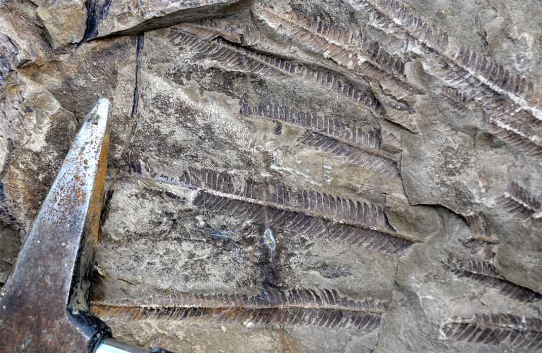
Fossil Cladophlebis fern from New Zealand Jurassic
These are all modelling results. They are calculating what the level of CO2 ought to have been given our knowledge of the Earth as a system. But for confirmation, we need ways to actually measure it. For the deep past we can’t do this directly, but instead we use ‘proxies’. These are measurements of some factor that responds to the level of CO2. One of these is the density of pores on the surface of leaves. CO2 is ‘breathed’ into plants by pores (stomata) scattered over their leaves. Their density is known to change with the amount of atmospheric CO2. When fossils leaves are preserved well-enough, their pore density can be measured, and the CO2 levels that they grew under, determined.
Some chemical reactions involving soil minerals, such as carbonate and iron oxides, also reflect atmospheric CO2 levels, and can be used in a similar way to leaf pores (e.g. Cerling 1991; Ekart et al. 1999; Royer 2006; Retallack 2009).
Initially, the results from these various techniques ranged widely. But the techniques were refined, and by 2010, there was more confidence that the modelled and measured CO2 amounts were starting to agree with each other (Breecker et al. 2010; Royer 2010). The Jurassic levels seem to have fluctuated between about 500-1500 ppm. Using the stomatal density technique on a Jurassic conifer from Australia, and CO2 range of 750–975 ppm was estimated (Steinthorsdotiir and Vajda 2013).
But others were experimenting with different ways to estimate volcanicity – by using the total lengths of volcanic ‘arcs’ (Lee et al. 2015) or the lengths of the subduction zones in which sea floor is consumed (van der Meer et al. 2014). These techniques estimated Jurassic CO2 levels to be around 700-1500 ppm. So despite very different ways of approaching the issue, the results are converging.
It is likely that New Zealand’s Jurassic Curio Bay forest likely grew in an atmosphere with CO2– levels at least three times what they were in pre-industrial times (less than 300 ppm) and at least twice what they are today (over 400 ppm). These results are not wildly different from the BLAG estimate of over 30 years ago. That level goes a long way to explaining forest growth a high southern latitudes. It would have been a world devoid of any ice sheets; certainly no ice at sea level, and correspondingly far higher sea-levels.
Today, much of the Curio Bay fossil forest lies below high tide (Pole 1999). It is sobering to realise that even with today’s CO2 levels, it is doomed to disappear below the waves.
References
Berner, R.A., (1991). A model for atmospheric CO2 over Phanerozoic time. American Journal of Science 291: 339-376.
Cerling TE (1991) Carbon dioxide in the atmosphere: Evidence from Cenozoic and Mesozoic paleosols. Am J Sci, 291: 377–400.
Ekart DD, Cerling TE, Montañez IP, Tabor NJ (1999) A 400 million year carbon isotope record of pedogenic carbonate: Implications for paleoatmospheric carbon dioxide. Am JSci, 299: 805–827.
Lee, C.-T.A., Thurner, S., Paterson, S., Cao, W., 2015. The rise and fall of continental arcs: Interplays between magmatism, uplift, weathering, and climate. Earth and Planetary Science Letters 425, 105–119.
Meer, D.G.van der, Zeebe, R.E., Hinsbergen, D.J.J.van, Sluijs, A., Spakman, W., Torsvik, T.H., 2014. Plate tectonic controls on atmospheric CO2 levels since the Triassic. PNAS 111: 4380–4385.
Retallack G (2009) Refining a pedogenic-carbonate CO2 paleobarometer to quantify a middle Miocene greenhouse spike.Palaeogeogr Palaeocl, 281: 57–65
Royer DL (2006) CO2-forced climate thresholds during the Phanerozoic. Geochim Cosmochim Acta, 70: 5665–5675
Royer, D.L., (2010). Fossil soils constrain ancient climate sensitivity. PNAS 107: 517–518.